
Something has bothered us since PGGB’s earliest days. With windowed sinc filters, we heard improvements as the filters grew longer. As we explored new upsampling approaches, that pattern never really went away — longer tracks still produced audible improvements, even when the underlying methods changed.
Those gains with longer filters made us wonder how much of the additional computation was actually contributing to what we heard, and whether the same result could be achieved with shorter filters and less sensitivity to window design.
The behavior of these filters is well understood. Here, we use measurements to show where their reconstruction errors occur and explain how PGGB’s new Precision Optimized Upsampling Engine addresses them.
The same length can give different accuracy.
Upsampling calculates additional samples between the original samples. The filter determines how those new values are calculated. Its individual weights are called coefficients, or taps. For a sinc-based filter, these weights are derived from the sinc function: we call them sinc coefficients (sinc coeffs). A window adjusts those weights; it does not change the sinc function itself.
An ideal sinc filter extends forever. A practical filter has to stop somewhere. An abrupt cutoff introduces reconstruction error. A window controls how the coefficients approach the ends. Some windows gradually reduce the coefficients across the whole filter. Others have a flat region in the middle where the sinc coeffs stay unchanged. How windowed-sinc filters work.

A weight of one leaves a sinc coeff unchanged. Lower weights reduce it. Rectangular stays flat and ends abruptly; Kaiser tapers across the window; Tukey keeps a flat middle with a taper at each end. The PGGB panel is an illustrative example, not the actual window design or the window used for the measurements. These are window shapes, not the sinc waveform itself.
Different choices produce different errors, even when the number of taps stays the same. The comparison below uses about 260k taps for each filter.
What does reconstruction accuracy mean?
Think of upsampling as filling in additional sample values between the ones already in the recording. Interpolation is the calculation used to find those values. Reconstruction accuracy asks how close those calculated values come to the ideal result.
We can generate a digital test signal directly at the higher sample rate. We can also generate the same signal at the original rate and upsample it. Comparing the two tells us how accurately the upsampler filled in the new samples. The difference is the reconstruction error: smaller errors mean more accurate upsampling.
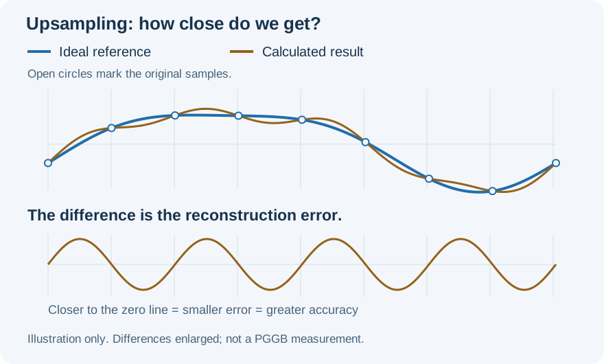
The bluesilver line is the ideal reference; gold shows a calculated result. The lower panel shows only their difference, enlarged so it is easy to see. This is a conceptual illustration, not measured PGGB performance. More plain-language definitions.
We express these errors as bits of reconstruction accuracy. One extra bit means half the error. Our measurement includes two contributions: unwanted copies of the music signal introduced during upsampling, called images, and errors in the signal we want to keep. It describes mathematical reconstruction before the output is rounded to its final bit depth.
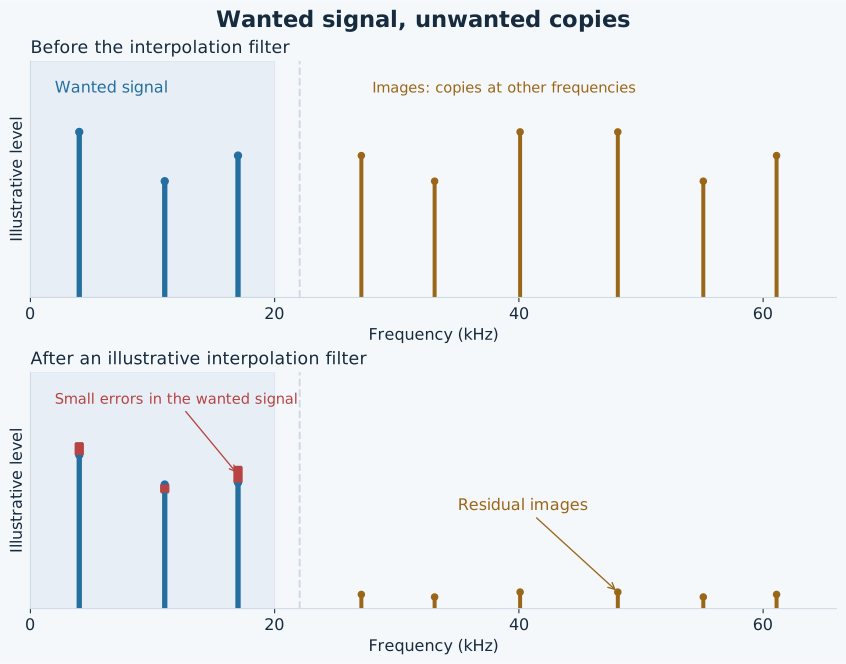
BlueSilver shows the wanted signal. Gold shows unwanted copies at other frequencies, called images. After filtering, any remaining images and errors in the wanted signal both count toward reconstruction error. This is a simplified illustration with exaggerated errors, not a measurement of PGGB or its HF filter. An introduction to spectral images and interpolation filtering.
For this blog, we use a 44.1 kHz input sample rate and report two regions: Audible band: DC–20 kHz and Extended band: 20–22 kHz. DC means zero frequency. The same principles apply at other sample rates, but the frequency boundaries and numerical results change with the rate.
Why stop at 22 kHz? At 44.1 kHz, Nyquist is 22.05 kHz. Accuracy falls rapidly as we approach that boundary. Maintaining very high accuracy ever closer to it requires increasingly long filters, eventually becoming impractical. Stopping 50 Hz short lets us make a useful comparison without implying the same accuracy right up to Nyquist. Background on filter length and transition width.

Different Windows, Same Length: about 260k taps. Higher means more accurate. The bars show measured values; labels are rounded down to two decimal places, so the measured band accuracy exceeds them. The result tables round to the nearest bit. View the equal-length window results and test conditions.
Keeping more sinc coeffs unchanged.
For the same filter length, the Tukey window provides greater reconstruction accuracy through 20 kHz, the conventional upper limit of the audible band, than the Kaiser and rectangular windows tested. The Kaiser window performs better in the 20–22 kHz band, while the rectangular window has the lowest accuracy in both measured bands. View our equal-length comparison results.
The Tukey window combines a flat middle with a gradual taper at each end. Compared with the tested Kaiser window, it leaves more sinc coeffs unchanged. Compared with the rectangular window, it avoids an abrupt ending.
That combination works well in this comparison. It does not mean that simply increasing the flat area will always improve a filter. The way the filter ends matters too.
A better taper can go further.
A different taper can improve accuracy without increasing either the total length or the number of unchanged sinc coeffs. Comparing the PGGB window with Tukey at about 260k taps each, while keeping the same number of unchanged sinc coeffs, shows the contribution of the window design.
In this comparison, the PGGB window reaches about 207 bits of accuracy through 20 kHz, compared with about 28 bits for Tukey. That is a substantial improvement without adding more taps or more unchanged sinc coeffs.
The result also has a boundary. Between 20 and 22 kHz, this PGGB window configuration is less accurate than Tukey. That distinction matters when we consider the listening results later.

Both filters have about 260k taps and the same number of unchanged sinc coeffs. The window design determines how the remaining coefficients taper toward the ends. View the equal-length window results and test conditions.
What happens when we keep adding sinc coeffs?
To show the effect of length alone, this comparison holds the PGGB taper fixed and adds unchanged sinc coeffs in the middle. This separates the benefit of additional sinc coeffs from the benefit of a longer taper.
Doubling the total length gives approximately one extra bit of accuracy in this comparison. Across two doublings, from one million to four million taps, the improvement is about 13 dB through 20 kHz and 11 dB over 20–22 kHz. That is close to two bits overall. Going from one million to four million taps therefore reduced reconstruction error by roughly a factor of four in each measured band.
Adding more unchanged sinc coeffs is beneficial, but it is a slow way to improve reconstruction accuracy. If the roughly one-bit-per-doubling trend continued, gaining another 30 bits would require about 2³⁰ times as many taps—roughly a billionfold increase in filter length. This is an extrapolation of the measured trend, not a measurement at that length.
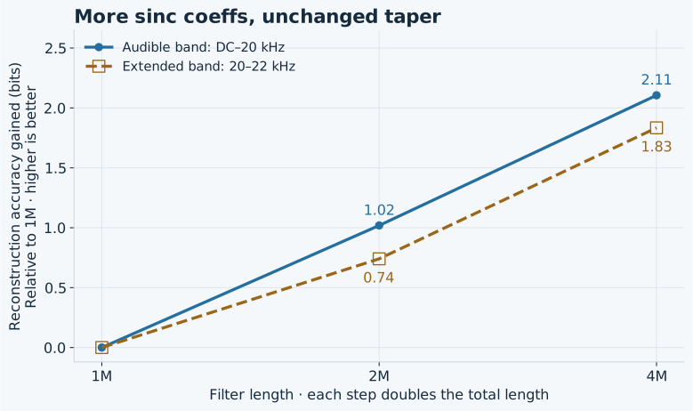
Each curve starts at the one-million-tap result. These gains apply to this fixed-taper comparison; they are not a universal rule for every way of increasing filter length. View the fixed-taper length results.
PGGB’s earlier move to FFT-based upsampling with the Nyquist–Shannon engine reduced its dependence on window design and provided the equivalent of very long sinc filters. That approach remained in use through V8. V8 did not use the window construction tested here. Yet we still heard improvements with longer tracks. The new engine addresses that remaining dependence by choosing filter lengths around the precision needed in the audible band.
Where could those benefits from longer filters be coming from?
For a 44.1 kHz recording, the Nyquist frequency is 22.05 kHz. This is the upper boundary set by its sample rate. Reconstruction becomes more demanding as we approach that boundary.
The two measurement bands make an important distinction visible. Through 20 kHz, a filter’s reconstruction error can already be below the numerical error level of the processing, leaving little practical benefit from further improvements there. Between 20 and 22 kHz, however, reconstruction error can still be much larger. Increasing length continues to improve this extended frequency region, just above the conventional audible band.
One possible explanation for the listening observations is that the remaining differences we hear are associated with the upper frequency band, potentially becoming audible through signal-correlated distortion, even when accuracy through 20 kHz has reached the useful limit of the working precision.
The measurements establish where the numerical differences lie. Listening tests address a different question: whether those differences change what we hear. The numerical results alone do not establish audibility or its cause.

These are filter-design errors calculated at high precision, before output quantization. Working precision places a separate limit on how accurately the processing can be performed. Read how reconstruction error is expressed in bits.
What the listening tests show.
A simple listening comparison can help explore whether the upper frequency band affects what we hear. In our listening tests, we used low-pass filtering to greatly reduce the contribution of the 20–22 kHz region while preserving the band through 20 kHz.
Listening tests by us and our testers revealed that the sound no longer changed with filter length or window parameters, provided reconstruction error in the retained band remained below the numerical error level of the processing. We also heard a significant improvement in sound quality compared with listening without the low-pass filter.
These listening results support the design approach: control the unwanted upper frequency band and provide the accuracy needed in the audible band.
Perfect upsampling: designing around precision.
That is the principle behind PGGB’s new Precision Optimized Upsampling Engine: choose a filter whose reconstruction error is below the numerical error of the calculations in the band being preserved, while controlling the upper frequency band separately. Arithmetic precision then becomes the main limit on reconstruction accuracy. PGGB’s math engine works at up to 256-bit precision, allowing very small numerical differences to be retained with extremely little rounding error.
This allows much shorter filters, resulting in faster processing and dramatically lower memory use. In our listening experiments, extending filter lengths further had no effect once we handled the upper frequency band and matched reconstruction accuracy to the processing precision in the audible band. Applying the same treatment of the upper frequency band to our existing V8 engine gave us the same listening result.
The following examples show how compact the reconstruction filter can become when sized for accuracy through 20 kHz:
| Target accuracy through 20 kHz | Approximate filter length at 16× | Measured accuracy through 20 kHz (nearest bit) |
|---|---|---|
| 107 bits | ~50k taps | 109 bits |
| 128 bits | ~60k taps | 130 bits |
| 256 bits | ~200k taps | 262 bits |
These numerically verified examples use our sizing method. They describe the reconstruction filter, not the combined size or cost of every processing stage. View the compact-filter results in both bands.
A short glossary.
| Term | Plain-language meaning |
|---|---|
| Upsampling | Increasing the sample rate by calculating extra sample values between the existing ones. It does not recover musical information that was never recorded. |
| Interpolation | The calculation used to fill in those additional sample values. Good interpolation follows the waveform represented by the original samples. |
| Ideal reference | The result we compare against: ideal reconstruction under the band-limited sampling model. It is a mathematical reference, not a separate recording of the performance. |
| Sinc function | The mathematical shape used for ideal reconstruction of a band-limited signal. Its ideal form extends indefinitely. |
| Sinc coefficients (sinc coeffs) | Filter weights derived from the sinc function. A window can leave some unchanged and taper others toward zero. |
| Tap or coefficient | One of the weights used by a filter to calculate its output. |
| Window and taper | A window shapes the filter’s coefficients. Its taper is the part that gradually reduces them toward the ends. |
| Flat region | The part of a window that leaves the underlying sinc coeffs unchanged. |
| Reconstruction accuracy | How closely the upsampled values match the ideal reference. You can think of it as the accuracy of the interpolation. Closer values mean greater accuracy. |
| Reconstruction error | The difference between a calculated value and the ideal value at the same instant. Our reported error also accounts for unwanted spectral copies introduced by upsampling. |
| Bit of accuracy | A way of expressing error size. One extra bit means half the error, or about 6 dB less. |
| Image | An unwanted copy of the signal at other frequencies, introduced during upsampling. Here “image” means a spectral copy, not a picture. The interpolation filter suppresses these copies. |
| Passband | The frequency range a filter is intended to preserve. |
| Nyquist frequency | Half the sample rate: 22.05 kHz for 44.1 kHz audio. |
| Working precision and mantissa | Working precision is the number of significant binary digits retained in a calculation. The mantissa is the part of a floating-point number that holds those digits. |
| Quantization and rounding | Representing a value using a limited set of available values introduces a difference when the original value cannot be represented exactly. This can happen during processing and when creating the final output. |
Measurement results.
These are our numerical results for the filters discussed here. They are separate from the background references below and from the reported listening observations.
- Test conditions and measurement method — how the reference, interpolation phases and worst-band errors are evaluated.
- Equal-length window comparison — rectangular, Kaiser, Tukey and PGGB at about 260k taps.
- Adding sinc coeffs with a fixed taper — results from one million to four million taps.
- Compact filters and their two-band results — the 107-, 128- and 256-bit target examples.
- Independent higher-precision checks — how the numerical results were verified.
References and further reading.
These sources explain the public signal-processing principles used in this article. Our PGGB comparisons are documented in the measurement results above; these references do not establish the reported listening observations.
- Steven W. Smith — Strategy of the Windowed-Sinc. An introduction to the ideal sinc function, finite filters and windowing.
- Steven W. Smith — Designing the Filter. How filter length, cutoff and windowing enter a conventional filter design.
- MathWorks — Signal Upsampling and Interpolation Filtering. A visual explanation of spectral images and interpolation filtering.
- SciPy — Tukey window, Kaiser window and rectangular window. Definitions of the three standard windows illustrated here.
- David Goldberg — What Every Computer Scientist Should Know About Floating-Point Arithmetic. Background on finite precision and rounding error.