
The attack of a piano note, a plucked string or a drum strike helps give an instrument its character. These rapid changes are called transients. We want an upsampler to preserve and reproduce them accurately.
A concern sometimes raised is that FFT-based processing loses this timing information when it converts the music into frequencies. Another is that floating-point calculations introduce rounding errors, while integer calculations can be exact.
PGGB’s use of FFTs preserves the timing information. Rounding does occur, but its impact depends on the precision used. A few additional bits can make up for that rounding penalty. PGGB goes much further, supporting a full 256-bit mantissa: the part of a floating-point number that holds its significant digits.
Where does the timing go?
An FFT describes a block of audio as a combination of waves. It keeps both the strength (level) of each wave and how the waves line up in time. That alignment is called phase.
Think of a musical performance. Knowing which notes were played, and how loudly, is only part of the story. When they were played matters too. A spectrum display often shows only the strengths. The FFT keeps the alignment as well.
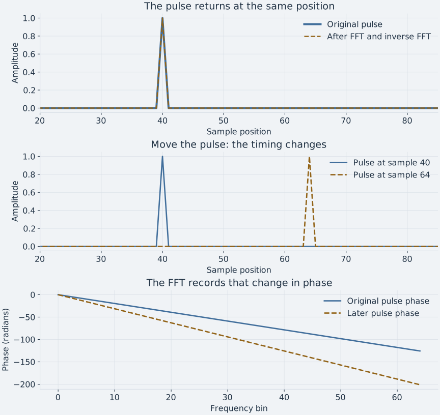
The pulse's position is preserved. Its timing is part of the information carried by the FFT. How phase carries a time shift.
Mathematical fact: With the same filter, correctly implemented FFT filtering and direct filtering calculate the same mathematical result. The filter determines how the waveform changes. The FFT provides an efficient way to calculate it. The convolution theorem explained.
What about rounding? All you need is 3 more bits!
Integer arithmetic can keep every product and sum exactly, provided there is enough room for the numbers. The running total is held in an accumulator; making it wide enough avoids losing information during the sum. Full-precision integer filtering.
Floating-point arithmetic keeps a limited number of significant digits. Think of a calculator with a limited display: a result that needs more digits must be rounded. Give the calculation more significant digits, and those rounding differences become smaller.
Each extra binary digit, or bit, halves the spacing between representable numbers at the same scale. A few more bits can therefore make a substantial difference.
For a simple comparison, let us assume an integer implementation delivers 104 bits of accuracy, with accumulators wide enough to support the calculation. Now allow roughly three bits for floating-point FFT rounding:
| Working precision | Approximate accuracy after the allowance |
|---|---|
| 104 significant bits | 101 bits |
| 107 significant bits | 104 bits |
| 256 significant bits | 253 bits |
On this simplified budget, about 107 bits of floating-point precision provides accuracy comparable to our assumed 104-bit integer calculation. Using only 104 floating-point bits would leave less accuracy after rounding.
The remedy is straightforward: allow a few extra bits for the calculation. PGGB's 256-bit mantissa provides far more working precision than this example requires.
What do the measurements show?
To measure rounding error, we filtered two kinds of signal: white noise, which contains a broad mix of frequencies, and a sequence of transients, made from short pulses and decaying oscillations. The transients included events crossing the boundaries between processing blocks.
For each test, we calculated the filtered signal using exact integer arithmetic. This reference kept every product and sum without rounding. We then calculated the same filter using an FFT, with exactly the same stored input samples and filter weights. The difference between the two outputs gives the FFT calculation's rounding error.
The tests covered nine filter lengths, doubling from 16,384 to 4,194,304 taps. A tap is one of the weights used by a filter. We used three working precisions and both common methods of joining processed blocks: overlap-add and overlap-save.
Here are the results for the four-million-tap filter. Each number expresses the largest sample error as bits of accuracy lost, relative to the filtered signal's peak. The table shows the larger error from the two block-processing methods.
| Working precision | White noise: bits lost | Transients: bits lost |
|---|---|---|
| 53 significant bits — IEEE64 | 2.67 | 0.59 |
| 113 significant bits — IEEE128 | 3.06 | 1.59 |
| 256 significant bits | 3.12 | 2.35 |
A loss of three bits has a different meaning depending on where we start. At 256-bit precision, it leaves roughly 253 bits of numerical accuracy on this measure.
Across all tested lengths, precisions and block methods, the largest loss was about 3.12 bits. The transient sequence had smaller peak-relative errors than white noise at every size and precision. These measurements support allowing roughly three extra bits for rounding in these calculations. PGGB goes above and beyond that allowance, all the way to 256 bits. Results for every filter length.
What this means for PGGB.
Floating-point rounding is real, and working precision gives us a direct way to reduce it. A few additional bits can compensate for the FFT's rounding penalty. PGGB supports up to 256 bits in the mantissa, the part of the number that carries its significant digits.
That precision is used during processing. It is separate from the output bit depth sent to your DAC.
The FFT has not discarded a transient that higher precision must somehow recover. It has retained the timing information throughout. Higher precision lets us calculate the filtered result more accurately.
The test setup and a closer look at the numbers
The nine filter lengths, three precisions, two signals and two block-processing methods give 108 test cases. Each uses a low-pass filter with the same design and an FFT twice the filter length. At four million taps, the FFT has 8,388,608 points. All 12,582,913 output samples are checked, including the filter's final tail.
IEEE64 calculations use MATLAB's 53-bit significant precision. IEEE128 calculations use Advanpix at 113 significant bits. The highest setting uses Advanpix with a true 256-bit mantissa. The sign and exponent account for the difference between an IEEE format's name and its significant precision.
The stored input samples use 24-bit fixed point and the filter weights use 32-bit fixed point. Exact integer convolution supplies the reference for these same stored values. Output differences are calculated at 665-bit precision, preserving errors far smaller than ordinary double precision could resolve at the signal's level. This comparison isolates rounding in the filter calculation.
For the table above, peak error is the largest absolute sample difference divided by the exact filtered signal's peak. The bit loss expresses this ratio relative to the calculation's working precision. One bit corresponds to approximately 6.02 dB: a 3.12-bit loss is about an 18.8 dB rounding penalty. The linked tables also provide RMS errors, which describe the overall error level rather than the largest sample difference.
Why a trillion times magnification is not enough.
To make the rounding differences visible, this close-up filters a 256-sample decaying oscillation with 49 filter weights and a 512-point FFT. Each result is compared with the exact integer reference. The four calculations use IEEE64, double-double (a leading double plus a correction), IEEE128 and a true 256-bit mantissa.
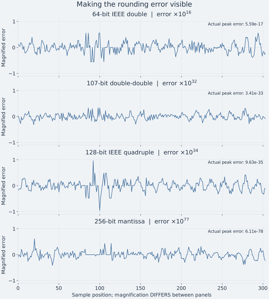
| Arithmetic | Largest absolute sample error | Magnification shown |
|---|---|---|
| IEEE64 | 5.59 × 10⁻¹⁷ | 10¹⁶ times |
| Double-double, approximately 107 bits | 3.41 × 10⁻³³ | 10³² times |
| IEEE128, 113 significant bits | 9.63 × 10⁻³⁵ | 10³⁴ times |
| True 256-bit mantissa | 6.11 × 10⁻⁷⁸ | 10⁷⁷ times |
A trillion is 10¹². The last panel uses a multiplier of 1 followed by 77 zeros. Each panel has a different scale; similar trace heights do not mean similar errors. The table gives the measured errors for this 49-tap illustration.
See the results by filter length, four-million-tap results and calculation validation for the full numerical tables and reference checks.
A short glossary.
| Term | What it means here |
|---|---|
| Sample | One stored value of an audio waveform. A sequence of samples describes how the waveform changes over time. |
| Transient | A rapid change in sound, such as the attack of a piano note or a drum strike. |
| FFT | Fast Fourier Transform: an efficient calculation that describes a block of samples as a combination of waves, keeping their levels and phase. An inverse FFT converts that description back into samples. |
| Phase | How a wave lines up in time. Together with its level, phase is needed to reconstruct the waveform. |
| Filter, taps and convolution | A filter combines weighted samples to shape a signal. The weights are called taps or coefficients. Applying those weights and adding the results is convolution. |
| Working precision | How many significant binary digits a calculation keeps. More precision allows smaller numerical differences to be represented. |
| Mantissa | The part of a floating-point number that holds its significant digits. The exponent sets the scale of the number. |
| Rounding error | The difference introduced when a calculated result needs more digits than the chosen precision can retain. |
| Accumulator | The running total used when adding the products in a filter calculation. It needs enough capacity to retain the required information. |
| Bits of accuracy | A way to express the size of an error relative to a stated reference. One extra bit means half the error, or about 6 dB less. This is separate from the number of bits in an output sample. |
| Peak and RMS error | Peak error is the largest difference. RMS, or root mean square, describes the overall level of the differences. The article states which measure each comparison uses. |
| Output bit depth | The number of bits used to store or send each output sample. It is separate from the precision used during processing. |
| Quantization | Representing a value using a limited set of available values. Rounding to an output bit depth is one example. |
| Overlap-add and overlap-save | Two ways to process audio in blocks and join the results so that the filter works correctly across block boundaries. |
References and further reading.
- Steven W. Smith — Fourier Transform Properties. Chapter 10 of The Scientist and Engineer's Guide to Digital Signal Processing. How phase carries a time shift while retaining the magnitude spectrum.
- Steven W. Smith — FFT Convolution. Chapter 18 of the same book. FFT filtering, block processing and the connection to direct convolution.
- MathWorks — Fixed-Point Precision Rules for Avoiding Overflow in FIR Filters. How sufficiently wide accumulators retain full-precision products and sums for stored inputs and coefficients.
- Clifford J. Weinstein — Roundoff noise in floating point fast Fourier transform computation. IEEE Transactions on Audio and Electroacoustics, AU-17(3), 209–215 (1969). A statistical model describing how FFT rounding noise grows with transform size.
- David Goldberg — What Every Computer Scientist Should Know About Floating-Point Arithmetic. Significant digits, rounding and numerical error.
- Yozo Hida, Xiaoye S. Li and David H. Bailey — Library for Double-Double and Quad-Double Arithmetic. Version dated May 8, 2008. How two IEEE doubles represent a higher-precision value, with at least 106 significant bits.
Measurement results.
Full numerical results and the checks used to establish the exact reference:
- Results by filter length: 16K to 4M taps — all 108 cases, with peak and RMS results and exact integer references.
- Actual four-million-tap results — measured endpoint details and reference validation.
- Calculation validation — precision settings and independent checks of the filter calculations.